Build a Dynamic Keyword Performance Report in Excel

This article will show you how to build an Excel worksheet that automatically filters its results after you enter one or more criteria.

My original goal was to analyze 2016 keyword performance for one of my company’s PPC accounts. For example:

• Which keywords had more than 3 conversions and a CPL below $30?
• Which keywords had a CPL above $100 and an average position above 3?
• Which keywords had between 1 and 3 conversions, a CPL above $150, and an average position below 3?

The file automatically lists the results matching the values entered above, as shown below:

 

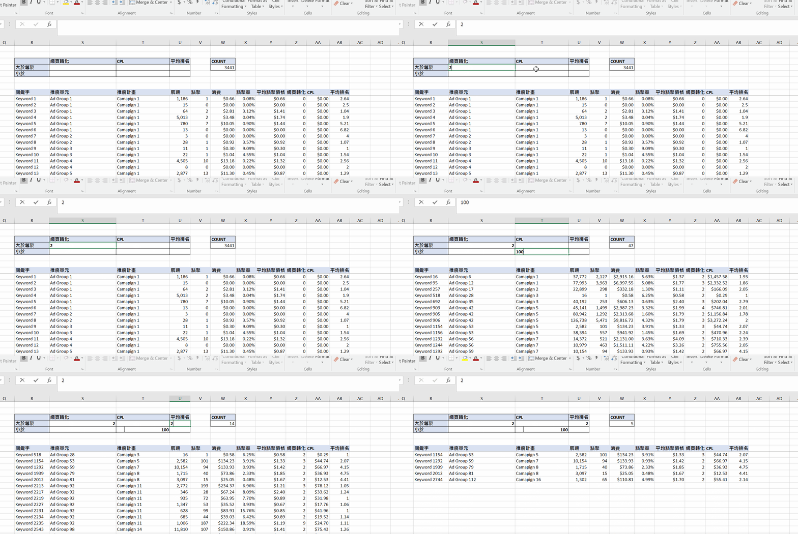
Although this example applies the method to paid-search keyword analysis, once you understand it, applying it elsewhere or adding more filter criteria will not be difficult! I will walk through the implementation step by step below. Download the file here!

Step One: Raw Data

The starting data looks perfectly ordinary, just like a typical export from AdWords or another tool. Because this was work-related, I replaced the real keywords, ad groups, and campaigns with other content~

(The client was a company in mainland China… so I used Simplified Chinese. Please excuse that!)

Step Two: Choose the Filter Criteria

Here, you need to think about how dividing the data would make the analysis useful. Some people may want to filter by CTR, while others may want to filter by time; there is no absolute right or wrong answer.

I chose website conversions, CPL, and position as the basis for my filters!

Step Three: Create Helper Column I

We need three helper columns to produce the result we want. The first helper column assigns a numeric ID to every keyword using this formula:

=ROWS($M$9:M9)

If you are wondering why we do not simply enter 1 in M8 and 2 in M9, then drag down to number every keyword, there is a reason! That method would cause problems if we added more rows to the source data later.

Step Four: Create Helper Column II*

Helper Column II is our criteria column, and it is the most important one.

We will begin with a simple condition. After confirming that it works, we will return and make the criteria more sophisticated.

The formula in N9 is:

=IF(J9>=$S$4,M9,"")

This means that if the value in the website conversions column (J) is greater than 1 (S4), the formula returns the value from Helper Column I (M); otherwise, it returns a blank ("").

The image above shows that when website conversions are greater than or equal to our chosen threshold, Helper Column II returns that keyword’s ID from Helper Column I. If we change S4 to 2, only keyword ID 1292 remains in Helper Column II.

Step Five: Create Helper Column III

The purpose of Helper Column III is to remove all the blank cells in Helper Column II, leaving only the IDs of keywords that meet the condition (more than 1 website conversion). The formula is:

=IFERROR(SMALL($N$9:$N$3449,M9),"")

In plain English, this formula selects the smallest value in column N for O9, the second-smallest for O10, the third-smallest for O11, and so on. After it reaches the largest value in column N—the last one that meets the criteria—it returns a blank ("").

If you already know the basics of Excel, you may have guessed the next step by now! The purpose of these three helper columns is to identify the rows containing every keyword that meets the criteria. The idea is the same as INDEX+MATCH: once we know which row each result is in, the dynamic table can use INDEX to retrieve the data.

Step Six: The Dynamic Table!

In this step, we build the final table that will be displayed. The formula uses INDEX, treating the source data as one large array, while HELPER3 lists the matching keywords one by one.

=INDEX($B$9:$O$3449,$O9,COLUMNS($R$9:R9))

1. $B$9:$O$3449 is the range containing all the source data, including the three helper columns.
2. $O9 is the number in Helper Column III—in other words, the row within this range that contains a keyword matching our criteria. We lock column O so that when we drag the formula to the right, it still looks only at the value in O, while dragging it down moves to the next matching keyword, and so on.
3. COLUMNS($R$9:R9) uses the same idea as Helper Column I. After we drag the formula to the right, column S displays Ad Group, T displays Campaign, U displays Impressions, and so on.

Finally, if INDEX does not find anything because the value that HELPER3 is looking for is blank, it returns an ugly #VALUE! error. We therefore wrap it in IFERROR so that the formula returns “” when INDEX finds nothing. The final formula is:

=IFERROR(INDEX($B$9:$O$3449,$O9,COLUMNS($R$9:R9)),"")

Step Six: Add More Filter Criteria

At this point, our dynamic worksheet is complete, but it can currently evaluate only one “condition”: it can select only website conversions greater than or equal to the number in S4. That is not especially useful, so we need to return to Helper Column II and enhance its formula so that it can evaluate multiple conditions at once.

=IF(J9>=$S$4,M9,"")

The formula above contains only one condition: whether J9 is greater than or equal to S4. To add more conditions in Excel, we simply use the AND and OR functions:

AND

Suppose we want to filter for results with at least 2 but fewer than 4 website conversions. The formula in Helper Column II becomes the following. Only when both J9>=$S$4 and J9<$S$5 are true does the IF formula return M9; otherwise, it returns a blank (“”).

=IF(AND(J9>=$S$4,J9<$S$5),M9,"")

OR

The formula above has a small bug. When no value is entered in S5, the number in column J will always be greater than the blank cell (""). Suppose a keyword has 3 conversions, we enter 2 in S4, and leave S5 blank. AND(3>=S4,3<S5) returns FALSE because the conversions column (J) in the source data always contains a number (0, 1, 2, 3, 4, and so on), and a number will always be considered greater than a blank cell.

To avoid this result, we can make the formula above slightly more complex:

=IF(AND(J9>=$S$4,OR(J9<$S$5,$S$5=""),M9,"")

Now the condition OR(J9<$S$5,$S$5="") returns TRUE when S5 is blank, because an OR expression is true whenever either of its two conditions is true ($S$5="").

Mix

Once we know how to use AND and OR, we can add as many comparison criteria as we want. At the beginning of the article, I selected three values to compare, so the final formula in Helper Column II becomes:

=IF(AND(J9>=$S$4,OR(J9<$S$5,$S$5=""),K9>=$T$4,OR(K9<$T$5,$T$5=""),L9>$U$4,OR(L9<$U$5,$U$5="")),M9,"")

It looks a little complicated, but this string is nothing more than a combination of AND and OR expressions that ultimately returns either TRUE or FALSE.

Step Seven: A Few Simple Improvements

That brings the main work to an end. Everything left is just a matter of simple refinement and appearance. You can hide columns A through O because users do not need to see them.

You can also add a “count” at the top so that users can clearly see how many keywords meet the selected criteria. The formula is:

=COUNTIF(R9:R3449,"?*")

Summary

I would not claim that this is absolutely the best method, but it is a small lesson from my own work that I wanted to share. I hope it comes in handy for you someday. If you have questions, suggestions, or feedback, feel free to leave a comment below or email me. Thank you for reading!